
Filters | communication systems laboratory experiment
Introduction
The Filtering process is an important part in any communication process especially in the Radio Spectrum .and it depends on being able to select one information-bearing signal from another, for example. Basically, a filter of the type used in this experiment allows energy at some frequencies to pass through and attenuates energy at other frequencies to a greater or lesser degree.
There are many forms of filter, indeed there are nearly as many different filters as there are ways of drawing an attenuation/frequency response. Of course a very common requirement is to have a single flat pass-band, and to cut off from the edges of the pass-band to a high attenuation stop-band in as few cycles as possible. The theory of sharp cut-off filters with extra attributes such as flat phase characteristics is beyond the scope of these experiments.
The objective here is to commence from the point of view that the basic filter comprises a combination of inductors and capacitors, and that more complicated filters connection. Three impedances in a four-terminal network can be placed in two configurations, designated here by π and T as shown in the next figure
The equivalence between these is demonstrated in the first experiment, which also introduces the idea of characteristic impedance Zo. If Zo is the same for two four-terminal networks at all frequencies of interest they may be connected in series, and in the second experiment reactive elements of the basic three-impedance type are investigated to show the constraints in the relationship between the network elements.
The following additional equipment is required:
comprising resistances or pure reactance's may be represented as an equivalent rr-section.
The importance of the characteristic impedance is also demonstrated.
Figure 10:1 shows a T and a n network, where Z stands for impedance, Y for admittance.
These two networks are equivalent if the following relations are applicable:
Zc = (Z1*Z2)/ZT , Zb = (Z2*Z3)/ZT , Za = (Z1*Z3)/ZT
Or consequently ,
Y3 = (Ya*Yb)/YT , Y2 = (Yb * Yc)/YT , Y1 = (Ya*Yc)/YT ;
If the sections are symmetrical, i.e. then the characteristic impedance is defined as the impedance looking into the input terminals when the output terminals are terminated in this characteristic impedance. In terms of the values shown in Figure 10:3 the characteristic impedance Zo is given in equation (1).

Z0 = (Z1 * Z2 + 1/4 Z1²)¹៸² ……………….. (1)
Z0 is also given by equation (2):
Z0 = (Zoc * Zsc )¹៸²
If the networks have the same characteristic impedance, they may be connected in cascade and treated as separate units, provided the cascaded sections are terminated in Zo.
Calculate the values of the impedances for the equivalent n for the two T sections given in the apparatus, one of which is purely resistive, the other purely reactive. Also calculate the characteristic impedance of each T-section over the frequency range 0 - 20kHz. The remainder of the experiment in this section will concentrate on the purely resistive n and T sections, which are generally referred to as attenuators.
In the logical build-up to more complex filters this T-section (or its equivalent n) is very
importam. It is one of the class of filters where the shunt and series impedances are connected by the relationship Zo *Z2 = Ro² where Ro is a real constant, and because of which it is known as a constant-k filter. It is also known as a prototype filter as other more complex filters can be derived from it (e.g. the m-derived filter dealt with later). Furthermore it has only one cut-off, where the characteristic impedance changes from real (pass) to imaginary (attenuation), see the calculations performed in the previous section.
Figure 04 shows low-pass constant-k T and n sections comprising the same series and
shunt impedances :

Their characteristic impedances are connected by equation (3).
ZOT / Zoπ = 1+ ( Z1 / 4Z2) …………. (3)
Where : Z1 : an Impedance L .
Z2 :a Capacitance C .
ZOT : is given by the equation (1) .
The cut-off Frequency of both the filters is given by the following equation :
ƒc = 1 / (π.(L*C)¹៸²) …………… (4)
Verify using (3) and (1) that both n and T sections have the same pass-bands. In the pass- band of the filter, it will be seen that although Zor is a pure resistance its value is a function of frequency. It is therefore impossible to terminate such a section correctly with a simple resistor. However Zo can be measured utilising equation (2).
Measure Zo for the constant-k low-pass T-section provided, by measuring the current into and voltage across the input to the constant-k section, the output of which is firstly short- circuited, and then open-circuited. Equation (2) can be used to compute Zor. This measurement should be performed at frequencies at 1kHz intervals over the pass-band.
(b) Have the same Z, as the prototype to allow ease of cascading.
(c) Have the same cut-off frequency.
A very simple class of filters meets all these requirements and is derived bv starting by multiplying the series impedance in the prototype T by m. Figure 10:6 (a) shows the required m-derived T section with its prototype, and which meets all the above requirements. By analogy, the same treatment can be applied to the n section, see Figure05 ,06.
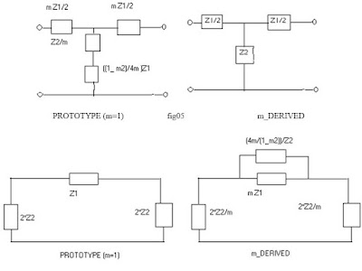
The problem of matching a constant-k section is overcome to a large extent by using m-derived half sections as terminating steps from the initial T to a pure resistance. An m-derived half section for the T in Figure03 is shown in Figure 07(A). A half section has clearly different impedances looking from either pair of terminals. One will be the character impedance ofitsm-derived section, the other depends on m.

A value of M = 0 6 is found to give the best fit over the pass band if the section is used as an impedance match between the basic T section and a pure resistance.
The input impedance to the m-derived half section used appropriately in a filter network
is given by equation (5).
Zo(half) = R [ 1 - ( 1 – m²) * X²] / ( 1 - X² ) ;
Where X² = Z1 / 4Z2 ;
Measure the input impedance of the filter shown in Figure 10:8 using the same method as before. Measure the input impedance over the frequency range 0-11 kHz. Compare the results with equation (5).
M2 =1- (fc / f∞ )²
fc = cut-off frequency given by equation (4)
f∞ = frequency of maximum attenuation.
To match Z, of the filter sections into a constant resistance, m-derived sections are usually used with m = 0.6
To examine the circuit shown in Figure08, firstly measure the insertion loss/frequency characteristic of the constant-k section alone between 600S2 loads over the frequency range 1 to 50kHz, by the substitution method described in the attenuator section.

Thus for a particular frequency output from the signal generator the voltage across the loads with either the variable attenuator or filter section should be made identical. The attenuation of the attenuator is then equal to the insertion loss of the filter.


fc = 14.14 KHz
L = 9.55 mH
C = 53.1 nF


 |
| Fig-01 |
The equivalence between these is demonstrated in the first experiment, which also introduces the idea of characteristic impedance Zo. If Zo is the same for two four-terminal networks at all frequencies of interest they may be connected in series, and in the second experiment reactive elements of the basic three-impedance type are investigated to show the constraints in the relationship between the network elements.
The Required Equipment & Procedures
The equipment that shown in Figure 02 consists of passive elements connected together in a number of combinations, with facilities for inter-connecting these combinations. There are two attenuators. The remaining combinations allow the investigation of low-pass (reactive-element only) 'T' and 'IT' circuits, an equivalent m-derived section and all the necessary half-sections and matching circuits. By means of these circuits the attenuation and impedance of a number of standard filters can be investigated as a function of frequency.The following additional equipment is required:
- Audio Signal Generator
- Calibrated Attenuator
- Oscilloscope or Voltmeter
T to π Conversion
The objective of this part of the experiment is to show experimentally chat a T-sectioncomprising resistances or pure reactance's may be represented as an equivalent rr-section.
The importance of the characteristic impedance is also demonstrated.
Figure 10:1 shows a T and a n network, where Z stands for impedance, Y for admittance.
These two networks are equivalent if the following relations are applicable:
Zc = (Z1*Z2)/ZT , Zb = (Z2*Z3)/ZT , Za = (Z1*Z3)/ZT
Or consequently ,
Y3 = (Ya*Yb)/YT , Y2 = (Yb * Yc)/YT , Y1 = (Ya*Yc)/YT ;
Where : ZT = Z1 + Z2 + Z3 ;
YT = Ya + Yb + Yc ;
If the sections are symmetrical, i.e. then the characteristic impedance is defined as the impedance looking into the input terminals when the output terminals are terminated in this characteristic impedance. In terms of the values shown in Figure 10:3 the characteristic impedance Zo is given in equation (1).

Z0 = (Z1 * Z2 + 1/4 Z1²)¹៸² ……………….. (1)
Z0 is also given by equation (2):
Z0 = (Zoc * Zsc )¹៸²
Zoc = Impedance at ab for cd open circuit.
Zsc = Impedance at ab for cd short circuit.
Zsc = Impedance at ab for cd short circuit.
If the networks have the same characteristic impedance, they may be connected in cascade and treated as separate units, provided the cascaded sections are terminated in Zo.
Calculate the values of the impedances for the equivalent n for the two T sections given in the apparatus, one of which is purely resistive, the other purely reactive. Also calculate the characteristic impedance of each T-section over the frequency range 0 - 20kHz. The remainder of the experiment in this section will concentrate on the purely resistive n and T sections, which are generally referred to as attenuators.
Place a load of value equivalent to the characteristic impedance across the output terminals of the resistive T sections. Feed the input terminals from an oscillator. Without adjusting the level output controls, measure the power into the load at a number of frequencies e.g. at 1 kHz intervals over the range 1kHz - 10kHz. The load power can be measured by either using a voltmeter or oscilloscope across the load. Now put a variable attenuator (accurate to O.ldB) between the oscillator and load and vary the attenuator for each of the frequencies of interest to give the same power reading in the load as before. These readings of attenuation are the insertion loss of the network. The theoretical value of insertion loss may be calculated by using (he network of Figure03 and finding the ratio of voltage in V to voltage across Ro load.


Low-pass Prototype Filter
In the previous part of the experiment, a calculation was performed which demonstrated that using reactances instead of resistances in a T network gives a characteristic impedance which varies with frequency.In the logical build-up to more complex filters this T-section (or its equivalent n) is very
importam. It is one of the class of filters where the shunt and series impedances are connected by the relationship Zo *Z2 = Ro² where Ro is a real constant, and because of which it is known as a constant-k filter. It is also known as a prototype filter as other more complex filters can be derived from it (e.g. the m-derived filter dealt with later). Furthermore it has only one cut-off, where the characteristic impedance changes from real (pass) to imaginary (attenuation), see the calculations performed in the previous section.
Figure 04 shows low-pass constant-k T and n sections comprising the same series and
shunt impedances :
Their characteristic impedances are connected by equation (3).
ZOT / Zoπ = 1+ ( Z1 / 4Z2) …………. (3)
Where : Z1 : an Impedance L .
Z2 :a Capacitance C .
ZOT : is given by the equation (1) .
The cut-off Frequency of both the filters is given by the following equation :
ƒc = 1 / (π.(L*C)¹៸²) …………… (4)
Verify using (3) and (1) that both n and T sections have the same pass-bands. In the pass- band of the filter, it will be seen that although Zor is a pure resistance its value is a function of frequency. It is therefore impossible to terminate such a section correctly with a simple resistor. However Zo can be measured utilising equation (2).
Measure Zo for the constant-k low-pass T-section provided, by measuring the current into and voltage across the input to the constant-k section, the output of which is firstly short- circuited, and then open-circuited. Equation (2) can be used to compute Zor. This measurement should be performed at frequencies at 1kHz intervals over the pass-band.
The M-derived Filter Section :
The step in complexity beyond the prototype constant-k section would at least (a) Have a more rapid attenuation-frequency cut-off in the stop-band.(b) Have the same Z, as the prototype to allow ease of cascading.
(c) Have the same cut-off frequency.
A very simple class of filters meets all these requirements and is derived bv starting by multiplying the series impedance in the prototype T by m. Figure 10:6 (a) shows the required m-derived T section with its prototype, and which meets all the above requirements. By analogy, the same treatment can be applied to the n section, see Figure05 ,06.

The problem of matching a constant-k section is overcome to a large extent by using m-derived half sections as terminating steps from the initial T to a pure resistance. An m-derived half section for the T in Figure03 is shown in Figure 07(A). A half section has clearly different impedances looking from either pair of terminals. One will be the character impedance ofitsm-derived section, the other depends on m.

A value of M = 0 6 is found to give the best fit over the pass band if the section is used as an impedance match between the basic T section and a pure resistance.
The input impedance to the m-derived half section used appropriately in a filter network
is given by equation (5).
Zo(half) = R [ 1 - ( 1 – m²) * X²] / ( 1 - X² ) ;
Where X² = Z1 / 4Z2 ;
Measure the input impedance of the filter shown in Figure 10:8 using the same method as before. Measure the input impedance over the frequency range 0-11 kHz. Compare the results with equation (5).
Attenuation Characteristics of Constant-k and m-derived Filter Sections:
The object is to investigate the attenuation/frequency characteristics of the various combinations of sections comprising low pass filters in the apparatus. A particular value ofm will result in a maximum value of attenuation at some frequency in the attenuation band.M2 =1- (fc / f∞ )²
fc = cut-off frequency given by equation (4)
f∞ = frequency of maximum attenuation.
To match Z, of the filter sections into a constant resistance, m-derived sections are usually used with m = 0.6
To examine the circuit shown in Figure08, firstly measure the insertion loss/frequency characteristic of the constant-k section alone between 600S2 loads over the frequency range 1 to 50kHz, by the substitution method described in the attenuator section.

Thus for a particular frequency output from the signal generator the voltage across the loads with either the variable attenuator or filter section should be made identical. The attenuation of the attenuator is then equal to the insertion loss of the filter.
Results & Conclusions:
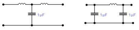
From the noticing of the experiments parts that we done in the laboratory ,we conclude the following:- For the first circuit that we wired which it is shown below , the output voltage will remains as it , and do not changed intend of changing the input frequency . We can notice that the output frequency will changed as in the input.

- For the second circuit that we wired in the laboratory which it is shown below , the output voltage will remain as it , and do not changed intend of changing the input frequency .

fc = 14.14 KHz
L = 9.55 mH
C = 53.1 nF
- You can see how the frequency effect in the output impedance. Testing the critical frequency of the low pass filter.


He is always engaged on new experiments, designs, and reviews and sharing his results on Tom's Hardware, YouTube, and extra. Once the mannequin has been sliced and the 3D printer has been ready, the next step is export the sliced mannequin as a .gcode file. The Creality Ender three Pro uses a microSD card for transferring .gcode recordsdata from your pc to the printer, and Creality Slicer will export the file directly to the card. This ready file was 5.8MB, which inserts easily on the 8GB microSD card which got here with the Ender three Pro. The steps right here are|listed beneath are} for the Creality Ender three Pro, however any 3D printer with a Bowden extruder will use an identical process for loading filament and calibrating Freediving Wetsuits For Women the build platform. You can see the distinction in the three Quickprint profiles in the above pictures .
ReplyDelete